Using the same engine makes it very easy to keep the global illumination in sync with the rest of the game. If we add new shaders or materials, change the representation of the geometry or alter the world, keeping the global illumination up to date requires little o no effort. Another interesting benefit is that optimizations to the rendering engine also benefit the global illumination pre-computation. However, as we will see later, in practice each application stresses the system in different ways and end up limited by different bottlenecks, what improves the rendering time does not necessary improve the pre-computation and vice-versa.
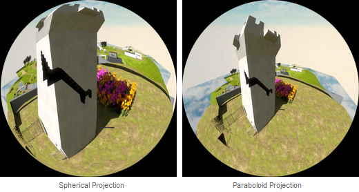
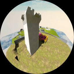
I tried several different approaches to render the scene and estimate the incoming radiance. The most common approach is to render hemicubes; that requires rendering the scene to 5 different viewports. Several sources suggested the use of spherical or parabolic projections, but in my experience these approaches produced terrible results due to the non linear projection. Without very high tessellation rates the scene would become unacceptably distorted, creating gaps between objects or making parallel surfaces self-intersect.
In
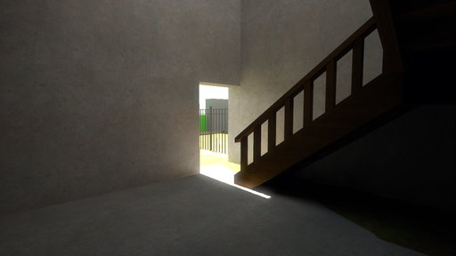
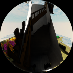
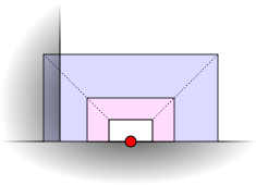
However, while this works OK from some points of view, the distortion becomes unacceptable when the camera is close to a surface, which is always our case. So, in practice these approaches are not very useful. Note how the outdoors are visible when sampling the lighting from the interior of the tower:
Other implementations use a single plane projection. This kind of projection does not capture the whole hemisphere, but by using a wide field of view it’s possible to capture about 80% of it. I haven’t actually tried this approach, but to get an idea of what the results would look like, I modified the hemicube integrator to ignore 20% of the samples near the horizon and found out that this introduced artifacts that were unacceptable for high-quality results.
estimates that on typical scenes this approach introduced a 18% RMS error, but suggests various tricks to reduce it by re-balancing the solid angle weights, or extrapolating the border samples and filling the holes. The latter method reduces the error down to a mere 6%.
However, these improvements do not eliminate banding artifacts caused when an intense light source visible from one location is suddenly not visible anymore in the next when it falls out of the projection frustum. To make things worse, the projection lacks rotational invariance, which enhances the problem when hemicubes are rendered with random rotations. So, while in many cases the results look alright, the few cases that do not render the method impractical.
Another problem is that the wide frustum is 4 times larger than the equivalent hemicube and easily intersects with the surrounding geometry; as I’ll discuss next, this is one of the main problems that I had to deal with.
In the end I simply stayed with the traditional hemicubes for simplicity. I think it would have been possible to do somewhat better using a fancy tetrahedral or pyramidal projection with 3 or 4 planes, but that didn’t seem worth the trouble.
As I just mentioned, one of the main problems that I had to solve was to handle overlaps between the hemicubes and the geometry. These overlaps are unavoidable unless you impose some severe modeling restrictions that are not desirable for production.
When the geometry is well formed and does not have self-intersections, these overlaps can sometimes be avoided with centroid sampling. Without centroid sampling the location where the hemicube is rendered from can easily end up being outside of the polygon that contains the sample and thus inside another volume.
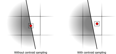
With centroid sampling the origin of the hemicube is now always inside the surface. However, it can still be very close to the surface boundary and have overlaps with nearby surfaces. A simple solution is to move the near plane closer to the camera until the overlap dissapears, but how close? The distance to the nearest boundary can be determined analytically, but there’s a limit in how much the near plane distance can be reduced without introducing depth sampling artifacts. An interesting solution for this problem is to render multiple hemicubes at the same location, each hemicube enclosing the previous one with its far plane at the near plane of the next.
That would solve most the problems when the geometry is watertight and centroid sampling is used, but in many cases our assets are not always well conditioned. So, I had to find a more general solution.
The extrapolation is not always correct, and the detection of invalid hemicubes is not 100% accurate, but so far this is the method that I’m happiest with. In the next article I’ll explain how this extrapolation is done in more detail.
Shadow Rendering
While the goal was to use the same rendering engine, using its shadow system ‘as is’ would have been overkill. We are using
Rasterization
Now that I’ve explained how to capture the irradiance of the scene at any point, it’s necessary to sample it for every lightmap texel. To do that I simply rasterize the geometry in the lightmap UV space using a conservative rasterizer and render one hemicube at every fragment whose coverage is above certain threshold.
This approach gives us a position and a direction to render the hemicube from, but I still need to determine the orientation of the hemicube. Initially, I simply chose an arbitrary orientation using
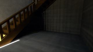
The source of the problem is just the limited hemicube resolution, but it’s surprisingly hard to get rid of it entirely by only increasing the hemicube size. A better solution is to simply use random orientations:
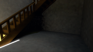
Note that I am trading banding artifacts by noise, but the latter is much easier to remove by using some smoothing.
Integration
Once the hemicubes have been rendered it’s necessary to integrate the sampled irradiance to compute the output radiance. The integral of the irradiance hemicube is simply a weighted sum of the samples, where the weights are the cosine-weighted areas of the hemicube texels projected on the hemisphere, that is, the cosine-weighted solid angles of the texels. These weights are constant, so they can be precomputed in advance.
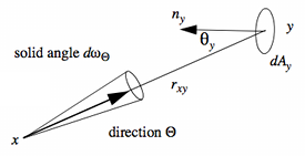
x and the center of the texel y
![]()
Asynchronous Memory Transfers
In the first place, you have to create two render targets and offscreen plain surfaces:
dev->CreateRenderTarget(..., &render_target_0);
dev->CreateRenderTarget(..., &render_target_1);
dev->CreateOffscreenPlainSurface(..., &offscreen_surface_0); dev->CreateOffscreenPlainSurface(..., &offscreen_surface_1);
The most important observation is that the only device method that appears to be asynchronous is GetRenderTargetData. After calling this method, any other device method blocks until the copy is complete. So, instead of overlapping the memory transfer with the rendering code, you have to find some CPU work to do simultaneously. In my case, I just do the integration of one of the render targets while copying the other:
while hemicubes left {
[...] // Render hemicube to render_target_0
// Initiate asynchronous copy to system memory.
dev->GetRenderTargetData(render_target_0, offscreen_surface_0);
// Lock offscreen_surface_1
// at this point the corresponding async copy has finished already.
offscreen_surface_1->LockRect(..., D3DLOCK_READONLY);
[...] // Integrate hemicube.
offscreen_surface_1->UnlockRect();
swap(render_target_0, render_target_1);
swap(offscreen_surface_0, offscreen_surface_1);
}
Another problem is that the buffer needs to be sufficiently big to reach transfer rates that saturate the available bandwidth. In order to achieve that I batch multiple hemicubes in a single texture atlas as seen in the following picture:
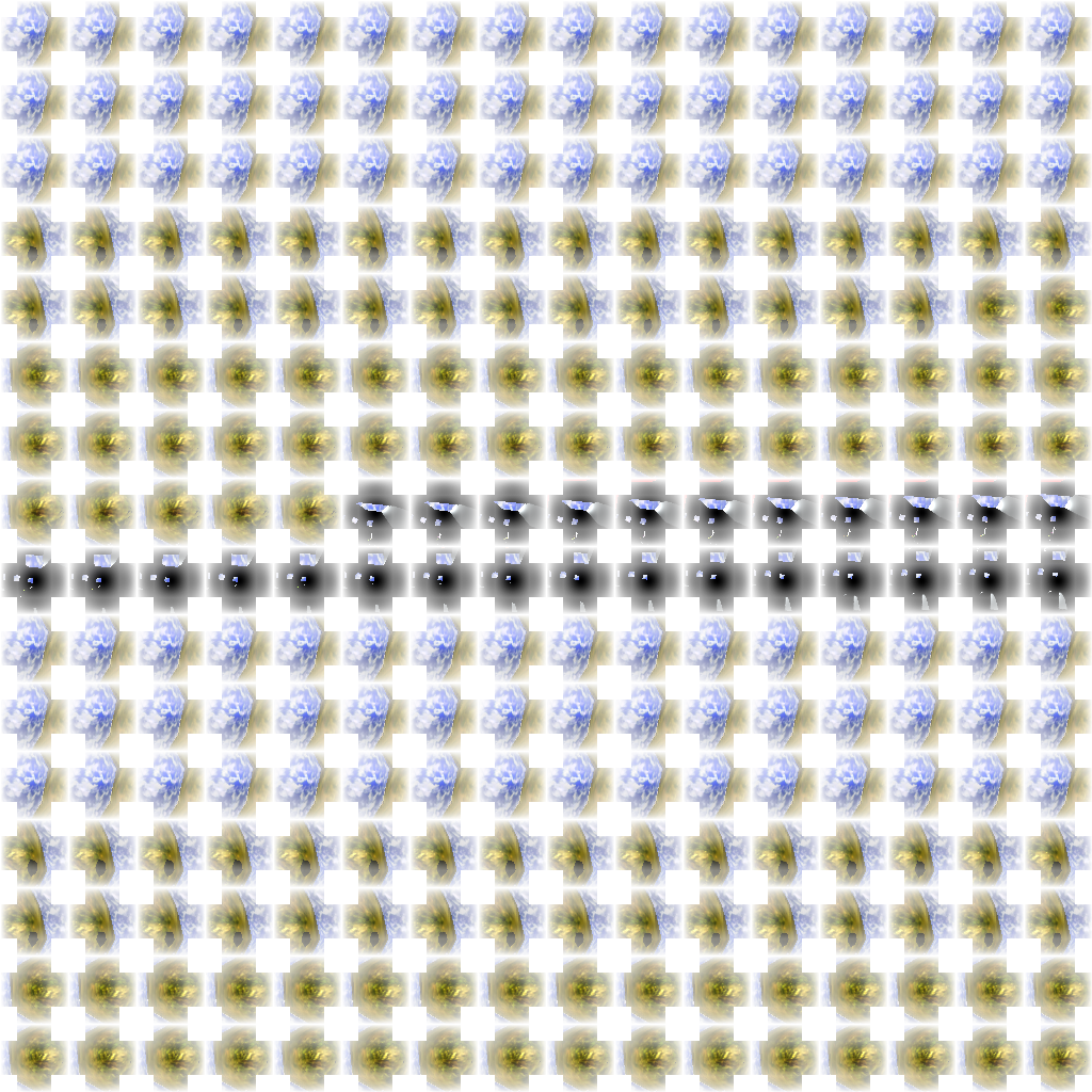
In practice I do not render the hemicubes using the depicted cross layout, but instead arrange the faces tightly in a 3×1 rectangle that does not waste any texture space and maximizes bandwidth. However, the cross layout was useful to visualize the output for debugging purposes.
Performance and Conclusions
The performance of our global illumination solution is somewhat disappointing. While we do most of the work on the GPU we are not really making a very effective use of it. The main GPU bottleneck is in the fixed function geometry pipeline; we are basically rendering a large number of tiny triangles on a small render target.
But that’s not the main problem. Traversing the scene in the CPU and submitting commands to render it actually takes more time than it takes the GPU to process the commands and render the scene, so the GPU is actually underutilized.
Our engine was designed for quick prototyping, to make it very easy to draw stuff with different materials, but not to do so in the most efficient way possible. These inefficiencies became a lot more pronounced in the lightmap baker.
On the bright side, as we optimize the CPU side of the engine we expect performance to improve. Modern GPUs also have functionality that make it possible to render to multiple hemicube faces at once. We expect that will also reduce the CPU work significantly.
While it was easy to get our global illumination solution up and running by reusing our rendering engine, bringing it to a level of sufficient quality and performance took a considerable amount of time. In the next installment I’ll describe some of the techniques and optimizations that I implemented to fix some of the remaining artifacts and improve performance.
Note: This article was originally published on The Witness blog.