Lightmap Compression in The Witness

In my initial implementation of our lightmapping technology I simply stored lightmap textures in RGBA16F format. This produced excellent results, but at a very high memory cost. I later switched to the R10G10B10A2 fixed point format to reduce the memory footprint of our lightmaps, but that introduced some quantization artifacts. At first glance it seemed that we would need more than 10 bits per component in order to have smooth gradients!

At the time the RGBM color transform seemed to be a popular way to encode lightmaps. I gave that a try and the results weren’t perfect, but it was a clear improvement and I could already think of several ways of improving the encoder. Over time I tested some of these ideas and managed to improve the quality significantly and also reduce the size of the lightmap data. In this post I’ll describe some of these ideas and support them with examples showing my results.

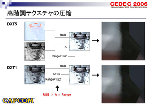I believe the RGBM transform was first proposed by Capcom in these CEDEC 2006 slides. While Capcom employs it for diffuse textures, it has become a popular way to encode lightmaps. RGBM or some of its variations are used in Unity, Bioshock Infinite, and the Unreal Engine, among others. Its use for standard color textures is not as widespread, but Shane Calimlim found it to be a good fit for the stylized artwork of Duck Tales and suggests it could be a good format in general. However, with so many precedents, I was surprised it had not been analyzed in more detail.

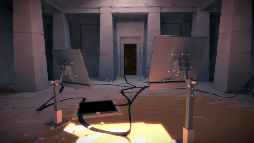
The main challenge of compressing lightmaps is that often they have a wider range than regular diffuse textures. This range is not as large as in typical HDR textures, but it’s large enough that using regular LDR formats results in obvious quantization artifacts. Lightmaps don’t usually have high frequency details, they are often close to greyscale, and only have smooth variations in the chrominance.

In our case, most our lightmap values are within the [0, 16] range, and in the rare occasions when they are outside of that range, we constrain them clamping the colors while preserving the hue to avoid saturation artifacts. Brian Karis also suggests tone mapping the upper section of the range to avoid sharp discontinuities, but I only found this to be a problem when light sources had unreasonably high intensity values.

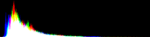
The shape of the lightmap color distribution varies considerably. Interior lightmaps are predominantly dark with a long tail of brighter highlights:

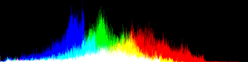
while outdoor lightmaps have a more Gaussian distribution with a bell-like shape. This particular lightmap is under the shade of some colored fall trees, which give it an orange tone:

Not all lightmaps use all the available range, so after tone mapping the next thing we do is to scale the range to [0, 1].

So, why is RGBM a good choice for data like this? The distribution of distinct values that can be represented with RGBM looks as follows:

It provides much more precision toward 0 than toward 1. This is beneficial for images that are intended to be visualized at multiple exposures. We want to obtain smooth lightmaps without quantization artifacts independently of the camera exposure. However, as we will see later, this provides much more precision around 0 than is actually necessary.

Naive RGBM Encoding

In my initial implementation I simply used RGBA8 textures, squaring the colors to perform gamma correction in the shader. The standard rgb -> RGBM transform is as follows:

m = max(r,g,b)
R = r/m
G = g/m
B = b/m
M = m

A simple improvement I did early on is to divide the quantization interval in two. This is a variation of the idea presented in Microsoft’s LUVW HDR texture paper, but instead of using an extra texture, I simply rely on the RGB and alpha (M) channels.

A similar observation is done by Shane Calimlim:

Gray is encoded as pure white in the color map, which may not always be optimal. Gray is an edge case most of the time, but a smarter encoding algorithm could make vast improvements in its handling. In the simple version of the algorithm the entire burden of representing gray lies with the multiply map; this could be split between both maps, improving precision greatly in scenarios where the color map can accommodate extra data without loss.

But in our case grey is not really an edge case! Lightmaps are mostly grey with slight smooth color variations.

The way I implemented this is by choosing a certain threshold t. For values of m that are lower than t the color is fully encoded using only the RGB components as follows:

R = r/t
G = g/t
B = b/t
M = 0

and for values of m greater than the threshold t, the normalized color is encoded in the RGB components, and the normalization factor m is biased and scaled to store it at a higher precision:

R = r/m
G = g/m
B = b/m
M = (m-t) / (1-t)

That’s equivalent to just doing:

m = max(r,g,b,t)
R = r/m
G = g/m
B = b/m
M = (m-t) / (1-t)

This is useful for several reasons. As Shane notes, splitting the burden of representing the luminance between the RGB and M maps we can obtain more precision and reduce the size of the quantization interval.

It’s important to note that this actually reduces precision around zero, where we don’t actually need so much, because the game camera never has long enough exposures. If we look at the distribution of grey levels that biased RGBM can represent it now looks as follows:

Picking different values of t allows us to use different quantization intervals for different parts of the color range. The optimal choice of t depends on the distribution of colors in the lightmap and the number of bits used to represent each of the components. We chose this value experimentally. For our lightmaps values around 0.3 seemed to work best when encoding them in RGBA8 format.

Optimized RGBM Encoding

With these improvements RGBM was already producing very good results. Visually I could not see any difference between the RGBM lightmaps and the raw half floating point lightmaps. However, I had not reduced the size of the lightmaps by much and ideally I wanted to compress them further.

The next thing that I tried to do was to choose M in a way that minimizes the quantization error. I did that by brute force, trying all possible values of M, computing the corresponding RGB values for that choice of M, and selecting the one that minimized the MSE:

for (int m = 0; m < 256; m++) {
    // Decode M
    float M = float(m) / 255.0f * (1 - threshold) + threshold;

    // Encode RGB.
    int R = ftoi_round(255.0f * saturate(r/ M));
    int G = ftoi_round(255.0f * saturate(g / M));
    int B = ftoi_round(255.0f * saturate(b / M));

    // Decode RGB.
    float dr = (float(R) / 255.0f) * M;
    float dg = (float(G) / 255.0f) * M;
    float db = (float(B) / 255.0f) * M;

    // Measure error.
    float error = square(r-dr) + square(g-dg) + square(b-db);

    if (error < bestError) {
        bestError = error;
        bestM = M;
    }
}

This improved the error substantially, but it introduced interpolation artifacts. The RGBM encoding is not linear, so interpolation of RGBM colors is not correct. With the naive method this was not a big deal, because adjacent texels usually had similar values of M, but the M values resulting from this optimization procedure were not necessarily similar anymore.

However, it was easy to solve this problem by constraining the search to a small range around the M value selected with the naive method:

float M = max(max(R, G), max(B, threshold));
int iM = ftoi_ceil((M - threshold) / (1 - threshold) * 255.0f);

for (int m = max(iM-16, 0); m < min(iM+16, 256); m++) {
    ...
}

This constrain did not reduce the quality noticeably, but eliminated the interpolation artifacts entirely.

While this idea showed that there's a significant optimization potential over the naive approach, it did not get us any closer to our stated goal: to reduce the size of the lightmaps. I tried to use a packed pixel format such as RGBA4, but even with the optimized encoding, it did not produce sufficiently high quality results. To reduce the size further we would have to use DXT block compression.

RGBM-DXT5

Simply compressing the RGBM data produced poor results and compressing the optimized RGBM data did not help, but instead only degraded the results even more.

A brute force compressor is not practical in this case, because when processing blocks of 4x4 colors simultaneously the search space is much larger.

A better approach is to first compress the RGB values obtained through the naive procedure using a standard DXT1 compressor and then choosing the M values to compensate for the quantization and compression errors of the DXT1 component.

That is, we want to compute M so that:

M * (R, G, B) == (r, g, b)

This gives us three equations that we can minimize in the least squares sense. The M that minimizes the error is:

M = dot(rgb, RGB) / dot(RGB, RGB)

In my tests, the resulting M's compress very well in the alpha map and reduced the error significantly.

I also tried to encode RGB again with the newly obtained M, and compress them afterward, but in most cases that did not improve the error. Something that worked well was to simply weight the RGB error by M in the initial compression step.

The number of bits allocated for the RGB and M components is very different than in our initial RGBA8 texture, so the choice of t had to be reviewed. In this case values of t around 0.15 produced best results. I attribute this to the reduced number of bits per pixel used to encode the RGB channels.

Results

In addition to the described formats I also compared the proposed method against BC6. BC6 is specifically designed to encode HDR textures, but it's not available in all hardware. Our optimized RGBM-DXT5 scheme provides nearly the same quality as BC6:

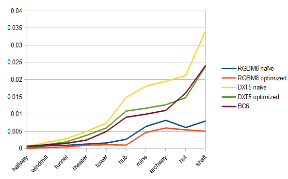
The above chart is displaying RMSE values of the final images after color space conversion and range rescaling.

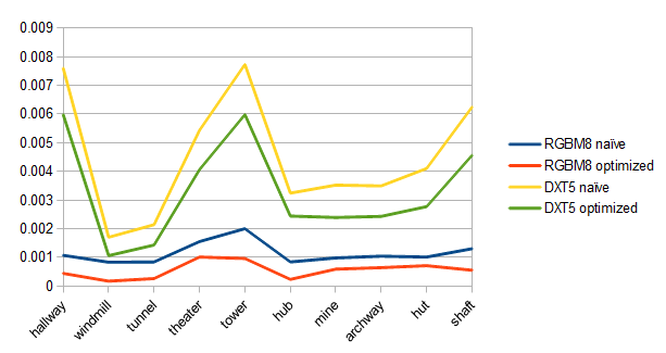
To study the effectiveness of the encoders it's more useful to look at the errors before rescaling. These look a lot more uniform, but cannot be compared against BC6 anymore, since in that case adjusting the range of the input values does not usually reduce the compression error.

Finally, I thought it would be interesting to use RGBM-DXT5 to compress standard images and compare it against YCoCg-DXT5. The following chart shows the results for the first 8 images of the kodim image set:

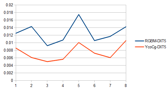
YCoCg-DXT5 is clearly a much better choice for LDR color textures.

Conclusions and Future Work

Our proposed RGBM encoder was good enough for our lightmaps, but I'm convinced there's more room for improvement.

One idea would be to pick a different threshold t for each texture. Finding the best t for a given texture to be encoded using the plain RGBM linear format would be easy, but it's not so obvious when using block compression.

The RGB components are encoded with a standard weighted DXT1 compressor. It would be interesting to use a specialized compressor that favored RGB values with errors that the M component could correct. For example, the M values resulting from the least squares minimization are sometimes above 1, but need to be clamped to the [0, 1] range, it should be possible to constrain the RGB endpoints to prevent that. It may also be possible to choose RGB endpoints such that the error of the least squares fitted M are as small as possible.

Finally, DXT5 is not available on most mobile GPUs. I haven't tried this yet, but it seems the ETC2 EAC_RGBA8 format is widely available and would be a good fit for the techniques presented here. It would also be interesting to compare our method against packed floating point formats such as (R11G11B10_FLOAT
R9G9B9E5_SHAREDEXP) and ASTC's HDR mode.

Tables

In all cases I measured the error using the RMSE metric, which is the same metric used to guide the block compressors. It may make more sense to use a metric that takes into account how the lightmaps are visualized in the game. I did exactly that, tone map the lightmaps at different exposures and compute the error in post-tone-mapping space. The tables below show the resulting values and they roughly correlate with the plain RMSE metric.

               Tone mapped error
            e=2.2   e=1.0   e=0.22     average   rmse

RGBM8 naive:

hallway:    0.00026 0.00045 0.00089 -> 0.00053 | 0.00007
hut:        0.00100 0.00102 0.00082 -> 0.00095 | 0.00609
archway:    0.00114 0.00141 0.00190 -> 0.00148 | 0.00818
windmill:   0.00102 0.00133 0.00185 -> 0.00140 | 0.00083
shaft:      0.00201 0.00228 0.00214 -> 0.00214 | 0.00798
hub:        0.00151 0.00182 0.00191 -> 0.00175 | 0.00267
tower:      0.00153 0.00200 0.00299 -> 0.00217 | 0.00160
tunnel:     0.00094 0.00123 0.00171 -> 0.00129 | 0.00093
mine:       0.00105 0.00120 0.00141 -> 0.00122 | 0.00640
theater:    0.00099 0.00126 0.00160 -> 0.00128 | 0.00129

RGBM8 optimized:

hallway     0.00010 0.00015 0.00030 -> 0.00018 | 0.00004
hut         0.00049 0.00043 0.00031 -> 0.00041 | 0.00543
archway     0.00044 0.00060 0.00122 -> 0.00075 | 0.00595
windmill    0.00020 0.00026 0.00036 -> 0.00027 | 0.00024
shaft       0.00059 0.00066 0.00102 -> 0.00076 | 0.00501
hub         0.00038 0.00051 0.00085 -> 0.00058 | 0.00099
tower       0.00060 0.00072 0.00082 -> 0.00072 | 0.00112
tunnel      0.00025 0.00031 0.00042 -> 0.00033 | 0.00048
mine:       0.00044 0.00049 0.00083 -> 0.00058 | 0.00467
theater:    0.00061 0.00076 0.00087 -> 0.00075 | 0.00095

RGBM4 optimized:

hallway:    0.00169 0.00259 0.00562 -> 0.00330 | 0.00063
hut:        0.00932 0.00899 0.00773 -> 0.00868 | 0.08317
archway:    0.00906 0.01287 0.02616 -> 0.01603 | 0.09614
windmill:   0.00424 0.00562 0.00830 -> 0.00606 | 0.00402
shaft:      0.01103 0.01314 0.01978 -> 0.01465 | 0.08204
hub:        0.00868 0.01160 0.01848 -> 0.01292 | 0.01722
tower:      0.01004 0.01217 0.01466 -> 0.01229 | 0.01835
tunnel:     0.00516 0.00687 0.01066 -> 0.00757 | 0.00764
mine:       0.00871 0.01044 0.01742 -> 0.01219 | 0.07510
theater:    0.00683 0.00840 0.00963 -> 0.00829 | 0.01057

DXT5 naive:

hallway:    0.00155 0.00249 0.00570 -> 0.00325 | 0.00048
hut:        0.00487 0.00536 0.00564 -> 0.00529 | 0.02119
archway:    0.00500 0.00656 0.01039 -> 0.00731 | 0.01949
windmill:   0.00214 0.00287 0.00444 -> 0.00315 | 0.00177
shaft:      0.01062 0.01339 0.01977 -> 0.01459 | 0.03412
hub:        0.00616 0.00796 0.01130 -> 0.00848 | 0.01481
tower:      0.00551 0.00712 0.01019 -> 0.00761 | 0.00735
tunnel:     0.00235 0.00308 0.00451 -> 0.00331 | 0.00285
mine:       0.00471 0.00589 0.00877 -> 0.00646 | 0.01809
theater:    0.00332 0.00412 0.00496 -> 0.00413 | 0.00498

DXT5 optimized:

hallway:    0.00125 0.00199 0.00456 -> 0.00260 | 0.00041
hut:        0.00336 0.00373 0.00408 -> 0.00372 | 0.01529
archway:    0.00353 0.00460 0.00719 -> 0.00511 | 0.01285
windmill:   0.00134 0.00180 0.00280 -> 0.00198 | 0.00116
shaft:      0.00801 0.01016 0.01507 -> 0.01108 | 0.02437
hub:        0.00469 0.00602 0.00846 -> 0.00639 | 0.01241
tower:      0.00421 0.00544 0.00781 -> 0.00582 | 0.00599
tunnel:     0.00157 0.00206 0.00306 -> 0.00223 | 0.00193
mine:       0.00338 0.00428 0.00646 -> 0.00471 | 0.01178
theater:    0.00245 0.00302 0.00357 -> 0.00301 | 0.00382

DXT5 optimized with M-weighted RGB:

hallway:    0.00114 0.00184 0.00430 -> 0.00243 | 0.00038
hut:        0.00338 0.00382 0.00443 -> 0.00388 | 0.01478
archway:    0.00356 0.00464 0.00725 -> 0.00515 | 0.01271
windmill:   0.00134 0.00180 0.00281 -> 0.00198 | 0.00113
shaft:      0.00804 0.01023 0.01522 -> 0.01116 | 0.02382
hub:        0.00472 0.00611 0.00868 -> 0.00650 | 0.01088
tower:      0.00421 0.00544 0.00787 -> 0.00584 | 0.00597
tunnel:     0.00157 0.00206 0.00306 -> 0.00223 | 0.00193
mine:       0.00337 0.00428 0.00648 -> 0.00471 | 0.01170
theater:    0.00245 0.00302 0.00356 -> 0.00301 | 0.00382