The NVIDIA Texture Tools (NVTT) had the highest quality BC1 encoder that was openly available, but the rest of the code was mediocre: The remaining encoders had not received much attention, the CUDA code paths were not maintained, and the accompanying image processing and serialization code was conventional. There was too much code that was not particularly interesting, it was a hassle to build, and required too much maintenance.
This compelled me to package the BC1 compressor independently as a single header library:
https://github.com/castano/icbc
While doing that I also took the opportunity to revisit the encoder and change the way it was vectorized. I wanted to write about that, but before getting into the details let’s overview how a BC1 compressor works.
Overview
A BC1 block is a 4×4 group texels that is represented with 2 16 bit colors and 16 2 bit indices. The colors are encoded in R5G6B5 format and define a 4 or 3 color palette. The entries of the palette are a convex combination of the 2 colors, for this reason they are usually referred as endpoints. The indices select one of the colors of the palette.
Nathan Reed provides a good overview of this and other block compression formats and Fabian Giesen has more lower level details about how the endpoints are interpolated on different GPU architectures.
In order to encode a BC1 block we need to choose the two endpoints 


In the 4 color block mode the values of 


If we know the index assigned to each texel, then we can solve the above equation system in the least squares sense and obtain the optimal values for the

That is, given a set of indices we need to compute two weighted sums of the colors, three weighted sums of the weights, and a 2×2 matrix inverse. An important observation is that if the indices are known in advance, the weighted sums of the weights is fixed and then the matrix inverse can be precomputed.
A simple BC1 encoding strategy is to compute the initial indices using a simple heuristic, to then recompute the endpoints solving the above equation, and finally to update the indices based on the most recent endpoints. This process can be repeated multiple times until the error does not go down anymore. This is the strategy employed by the stb_dxt.h encoder, and just as I was writing this article Fabien Giesen wrote another blog post describing that implementation in more detail.
Another approach would be to solve the optimization problem for all possible index combinations. In a 4×4 block with 2 bit indices per-texel the total number of possible index combinations is 
To count and enumerate the clusters that are possible with 16 indices and 4 colors we could use code like this:
cluster_count = 0
for c0: 0..15 {
  for c1: 0..15-c0 {
    for c2: 0..15-(c0 + c1) {
      cluster_count += 1
      c3 = 16 - (c0 + c1 + c2)
      println c0, c1, c2, c3
    }
  }
}
The number of resulting indices is just 969. Solving the resulting 969 equations gives us a nearly optimal solution. I say nearly, because the resulting endpoints $a, b$ are not stored exactly, but clamped and quantized. That is, in reality we have a discrete optimization problem (box-constrained integer least squares) and we are approximating it solving a continuous optimization problem and clamping and quantizing the solution.
The line that is used to determine the sort order of the colors is fairly important. The most obvious choice is to use the best fit line and that seems to work best in practice. It’s important to compute it with enough precision. I proposed to use power iterations in order to compute the direction of the first eigenvector of the covariance matrix, but this is very sensitive to the initial approximation. In an early implementation I simply used the ")
Simon Brown tried to repeat the optimization process by using the direction of the segment connecting the endpoints and repeating this iteratively, but in practice this often produced lower quality results than the solution found in the first iteration, so it’s not recommended.
This same process works with any numbers of clusters. For example, in the 3 color mode we have 3 clusters and the weights have the following values: 
cluster_count = 0
for c0: 0..15 {
  for c1: 0..15-c0 {
    cluster_count += 1
    c2 = 16 - (c0 + c1)
    println c0, c1, c2
  }
}
And in this case the result is much smaller, just 153. Even though the optimization cost is smaller, the 3 color mode rarely produces higher quality results than the 4 color mode, so the additional cost rarely justifies the effort unless you want to squeeze as much quality as possible out of the format.
That said, the 3 color mode shines when the block has texels close to black. The 4th color in this mode is used to represent transparencies. The alpha is expected to be premultiplied, and for this reason the corresponding RGB component is black. By ignoring all the texels that are near black, we can compute a best fit line that approximates the remaining colors much more accurately and that results in a much lower error. For this strategy to work, though, we need to be aware that the resulting texture may have unexpected alpha values. Some platforms allow us to swizzle the alpha to 255, but otherwise we have to be careful the shaders don’t assume opaque alpha.
For other formats with higher number of palette entries, this optimization strategy is not particularly useful as the number of cluster combinations goes up very quickly:
2 ->      17
3 ->     153
4 ->     969
5 ->   4,845
6 ->  20,349
7 ->  74,613
8 -> 245,157
One of the optimization strategies in Rich’s BC1 compressor (rgbcx) is to reduce the number of cluster combinations to be considered. If you compute a histogram to visualize the distribution of clusters, you will notice that some of them are much more likely to occur than others. By pruning the list of clusters it’s possible to trade quality for increased speed in the encoder. I do not employ this strategy for reasons that I’ll describe later.
So far I have assumed the hardware interpolates the colors using the ideal weights
Vectorization
In the original cluster fit implementation Simon and I used SSE2 and VMX instructions to speedup the solver. These vector instructions can operate on 4 floats at a time. We used them to operate on RGB colors and increased their utilization by storing weights in the alpha component and operating on them simultaneously. Readability of the code suffered and performance was only 2.3 times faster than the scalar implementation.
In that implementation we iterated over all the possible cluster combinations using three nested loops and incrementally computed the color sums that are necessary to solve the least squares system:
vec4 x0 = 0;
for c0: 0..15 {
  vec4 x1 = 0;
    for c1: 0..15-c0 {
      vec4 x2 = 0;
      for c2: 0..15-c1-c0 {
        alphax_sum = x0 + x1 * (2.0f / 3.0f) + x2 * (1.0f / 3.0f);
        ...
        x2 += color[c0+c1+c2];
      }
      x1 += color[c0+c1];
  }
  x0 += color[c0];
}
This worked well, but this approach didn’t scale to larger vector sizes that are increasingly common in current CPUs and the incremental nature of the computations created many pipeline dependencies.
In my CUDA implementation I used a different approach: I solved a least squares system on each thread. To do that I precomputed the indices of every cluster combination and loaded each one in a separate thread.
The incremental approach I used before was not possible in this setting, so instead I looped over the 16 colors in order to compute the corresponding sums:
parallel for i: 0..968 {
  indices = total_indices[i];
  alphax_sum = {0, 0, 0};
  for j: 0..15 {
    index = (indices >> (2*j)) & 0x3;
    alpha = weight(index);
    alphax_sum += alpha * colors[j];
    ...
  }
  ...
}
I was planning to do something along these lines when I revisited my CPU implementation, but instead I borrowed a trick from Rich Geldreich: to use summation tables to quickly compute partial color sums.
If we compute the sums of the sorted colors as follows:
color_sum[0] = { .r = 0, .g = 0, .b = 0 };
for (int i = 1; i <= color_count; i++) {
    color_sum[i].r = color_sum[i - 1].r + colors[i].r;
    color_sum[i].g = color_sum[i - 1].g + colors[i].g;
    color_sum[i].b = color_sum[i - 1].b + colors[i].b;
}
Then we can easily compute the partial sums of the colors in any of the clusters by subtracting two entries from that table:
parallel for i: 0..968 {
  c0, c1, c2 = total_clusters[i];
  x0 = color_sum[c0] - 0;
  x1 = color_sum[c1+c0] - color_sum[c0];
  x2 = color_sum[c2+c1+c0] - color_sum[c1+c0];
  alphax_sum = x0 + x1 * (2.0f / 3.0f) + x2 * (1.0f / 3.0f);
  ...
}
In practice we load the prefix sum of the cluster counts and compute the color sums with just a couple of subtractions.
parallel for i: 0..968 {
  c0, c1, c2 = total_clusters[i];
  x0 = color_sum[c0];
  x1 = color_sum[c1];
  x2 = color_sum[c2];
  x2 -= x1;
  x1 -= x0;
  alphax_sum = x0 + x1 * (2.0f / 3.0f) + x2 * (1.0f / 3.0f);
  ...
}
Note also that we don’t need to compute x3, the sum of the colors in the 4th cluster, because it’s only necessary in order to compute 
betax_sum = color_sum[15] - alphax_sumIn order to do this efficiently with vector instructions it’s necessary to lookup the values from the summation tables without falling back to scalar loads.
This can be done very easily with the AVX512 instruction set. The summation tables have 17 entries, but we know the first entry is always zero, so the entire table can be loaded in a 512 bit register, the index decreased by 1 and the loaded value zeroed when the index is negative. To perform the lookup we can use _mm512_maskz_permutexvar_ps and take advantage of the mask argument to zero the first index.
__m512 vfltmax = _mm512_set1_ps(FLT_MAX);
__m512 vr_sum = _mm512_mask_load_ps(vfltmax, loadmask, r_sum);
__m512 vg_sum = _mm512_mask_load_ps(vfltmax, loadmask, g_sum);
__m512 vb_sum = _mm512_mask_load_ps(vfltmax, loadmask, b_sum);

vx0.x = _mm512_maskz_permutexvar_ps(c0 >= 0, c0, vr_sum);
vx0.y = _mm512_maskz_permutexvar_ps(c0 >= 0, c0, vg_sum);
vx0.z = _mm512_maskz_permutexvar_ps(c0 >= 0, c0, vb_sum);

vx1.x = _mm512_maskz_permutexvar_ps(c1 >= 0, c1, vr_sum);
vx1.y = _mm512_maskz_permutexvar_ps(c1 >= 0, c1, vg_sum);
vx1.z = _mm512_maskz_permutexvar_ps(c1 >= 0, c1, vb_sum);

vx2.x = _mm512_maskz_permutexvar_ps(c2 >= 0, c2, vr_sum);
vx2.y = _mm512_maskz_permutexvar_ps(c2 >= 0, c2, vg_sum);
vx2.z = _mm512_maskz_permutexvar_ps(c2 >= 0, c2, vb_sum);
NEON does not have packed scalar permutes, nor 512 bit registers, but supports vqtbl4q_u8, a form of the TBL instruction that performs a vector lookup from 4 source registers. This is not as convenient as the AVX512 instruction, because it operates at the byte level. But that only means we need to do a bit more precomputation and transform the sums of cluster sums into byte offsets. Conveniently, if an index is out of range, the result for that lookup is 0, so we don’t have to worry about masking negative indices.
vx0.x = vreinterpretq_f32_u8(vqtbl4q_u8(r_sum, idx0));
vx0.y = vreinterpretq_f32_u8(vqtbl4q_u8(g_sum, idx0));
vx0.z = vreinterpretq_f32_u8(vqtbl4q_u8(b_sum, idx0));

vx1.x = vreinterpretq_f32_u8(vqtbl4q_u8(r_sum, idx1));
vx1.y = vreinterpretq_f32_u8(vqtbl4q_u8(g_sum, idx1));
vx1.z = vreinterpretq_f32_u8(vqtbl4q_u8(b_sum, idx1));

vx2.x = vreinterpretq_f32_u8(vqtbl4q_u8(r_sum, idx2));
vx2.y = vreinterpretq_f32_u8(vqtbl4q_u8(g_sum, idx2));
vx2.z = vreinterpretq_f32_u8(vqtbl4q_u8(b_sum, idx2));
At first I struggled to implement these with AVX2 and SSE2 instructions.
My first attempt with AVX2 to perform a masked lookup was to load the table in two registers, use _mm256_permutevar8x32_ps on each one, combine the result with _mm256_blendv_ps and mask the zero elements:
vlo = _mm256_permutevar8x32_ps(vlo, idx);
vhi = _mm256_permutevar8x32_ps(vhi, idx);
v = _mm256_blendv_ps(vlo, vhi, idx > 7);
v = _mm256_and_ps(v, mask);
This worked well, but Fabian Giesen pointed out that permutes and blends conflict for the same port and instead suggested to first xor the upper part of the table:
vhi = _mm256_xor_ps(vhi, vlo);So that the blend can be emulated with a sequence of cmp, and and xor:
vlo = _mm256_permutevar8x32_ps(vlo, idx);
vhi = _mm256_permutevar8x32_ps(vhi, idx);
v = _mm256_xor_ps(vlo, _mm256_and_ps(vhi, idx > 7));
v = _mm256_and_ps(v, mask);
This resulted in a significant speedup, but the cool thing is that the same idea extends to larger tables or to architectures with smaller register sizes. For example, in SSSE3 we can use the pshufb instruction with the same tables we used in the VTL NEON code path, but first we xor the upper part of the table as follow:
tab3 = _mm_xor_ps(tab3, tab2);
tab2 = _mm_xor_ps(tab2, tab1);
tab1 = _mm_xor_ps(tab1, tab0);
and then at runtime we can use pshufb to emulate our lookup combining multiple permutations:
v = _mm_shuffle_epi8(tab0, idx);
idx = _mm_sub_epi8(idx, _mm_set1_epi8(16));

v = _mm_xor_si128(v, _mm_shuffle_epi8(tab1, idx));
idx = _mm_sub_epi8(idx, _mm_set1_epi8(16));

v = _mm_xor_si128(v, _mm_shuffle_epi8(tab2, idx));
idx = _mm_sub_epi8(idx, _mm_set1_epi8(16));

v = _mm_xor_si128(v, _mm_shuffle_epi8(tab3, idx));
Note that pshufb sets the destination to zero when the second argument is negative. This eliminates the need to perform an and and a comparison as we did in the AVX2 case, and also handles automatically the indexing of the zero element of the summation table.
I’ve glossed over many of the implementation details to focus on the aspects that I think are most interesting, but if you are curious here’s the whole implementation.
Weighted Cluster Fit
An important difference between the ICBC compressor and most other compressors out there is that it supports per-texel weights. What this means is that rather than solving the least squares equation in the ordinary way, I scale the equation corresponding to each texel with the associated weight.
This improves the quality of alpha maps significantly allowing the compressor to approximate opaque texels much more accurately than transparent or semi-transparent ones. It’s also important when compressing lightmaps; texels outside of the chart footprint do not need to be considered by the compressor and can be ignored. This also offers a convenient way of supporting block sizes that are not exactly 4×4 and it’s also useful when compressing textures encoded in RGBM. Since the M multiplies the RGB components, the errors associated to texels with lower M values are less important than those associated to texels with high M values. Another application incorporate perceptual metrics to adjust these weight maps based on the smoothness or other features of the image.
On the other hand this introduces some additional cost. That’s is not just because you have to scale the
This is so much faster than evaluating the inverse, that for a while I maintained two versions of the code. One for use when the input was weighted and another when it wasn’t.
However, an advantage of the weighted cluster fit method that I initially overlooked is that color blocks often have some texels with the same value. In those cases, the number of colors in the block can be reduced and their weights adjusted accordingly. This improves performance significantly, because the number of cluster combinations depends on the number of input colors and grows faster than linearly:
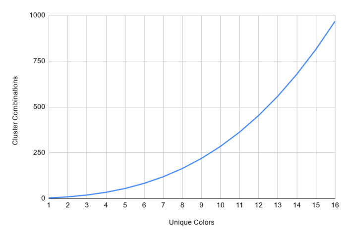
| Unique Colors | 1 | 2 | 3 | 4 | 5 | 6 | 7 | 8 | 9 | 10 | 11 | 12 | 13 | 14 | 15 | 16 |
|---|---|---|---|---|---|---|---|---|---|---|---|---|---|---|---|---|
| Cluster Combinations | 3 | 9 | 19 | 34 | 55 | 83 | 119 | 164 | 219 | 285 | 363 | 454 | 559 | 679 | 815 | 968 |
For example, with 16 colors there are 969 combinations, but with 12 colors there are 454 combinations (roughly half), and with 8 colors there are only 164 combinations (17% of the total). The precomputation method is only faster when the number of colors is exactly 16. With 15 colors the weighted method already runs at about the same speed and color blocks with 16 unique colors are actually very rare.
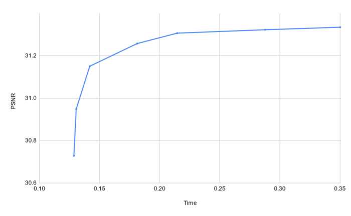
Finally, another interesting advantage of the weighted cluster fit method is that it also provides a simple way to adjust the quality of the output and reduce the time it takes to encode a block. The only thing that we need to do is to cluster or snap together some of the input colors to reduce the total number of colors in the block.
The following graph shows how the quality and compression time changes as we adjust the clustering threshold:
It may be possible to combine this strategy with Rich’s, but his requires precomputing subsets of cluster combinations that is specific to the number of colors in the block. With a variable number of colors the amount of data to tune and precompute would go up significantly.
Last words
There are many aspects of my implementation that are at bit sloppy and I’m sure it’s possible to squeeze a bit more performance out of it. Significant parts of the code are not vectorized, and this becomes very noticeable at low quality settings (look at all that empty space to the left of the curve in the graph above!). Algorithmic improvements are still possible, and I’ll be writing about some of them in the future.
The BC1 format is not particularly relevant today, but many of the techniques employed here can be useful in other settings. In modern formats such as BC7 and ASTC the search space is so much larger that most encoders don’t put a lot of effort into optimizing the solution for a specific partition or mode, some of these techniques can still be relevant.
“The BC1 format is not particularly relevant today” Except for literally every single pc game spare for 2d games that cannot use lossy compression, and a few weird engines that store images as .png instead of a gpu format? Its not going away until something else takes over the 4bpp range, and even then engines will take their sweet time and then some, much like how voxel cone traced GI still isnt a thing a decade later.