Irradiance Caching – Continued

Looks like I’m getting into the habit of starting article series and abandoning them after the first installment. Where’s part 2 of the irradiance caching article that I wrote several years ago? Before starting a new series, I think it’s about time to wrap that one up.

In the final part I wanted to write a bit about our record placement strategy. The main idea was to use the irradiance gradients to control the record density. That was nothing new, in Making Radiance and Irradiance Caching Practical Krivanek, et al also propose adjusting the record distribution based on the rate of change in the irradiance.

However, the interesting observation is that the scale of the gradient is not that relevant, what we care about are changes in the rate of change, that is, second order differences. If a sample has a small gradient and the one next to it has a large one, that’s an indication that the irradiance between the two changes abruptly and that additional samples may need to be taken in between them.

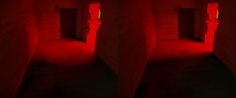
The way I took that into account when building our record distribution is using a procedure similar to the “neighbor clamping” algorithm described in the same paper. When a new record is inserted in the cache, I look up the neighboring records and if their gradients are significantly different, then I scale the records down to avoid overlaps and make space for additional samples in between them. The following picture shows the result of applying this procedure, you can hover the mouse cursor over it to see the actual records and their radius:

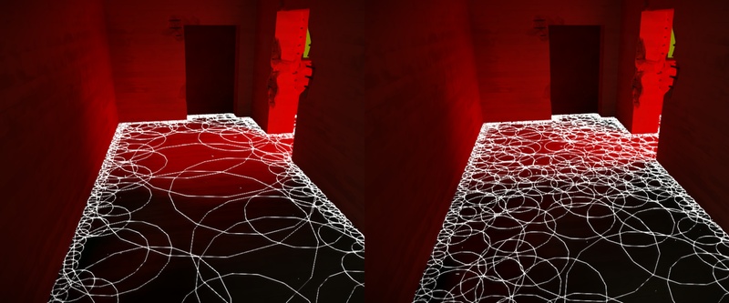
On the left is the original method that only uses the split sphere heuristic and the scale of the gradients to determine the record radius and placement. On the right is the method I propose, that adjusts the record scale based on the gradient differences. You can see that on the left side some of the records are too large and are “unaware” of the occlusion due to the wall, the resulting distribution is too sparse for the actual irradiance field and produce choppy results. These artifacts would eventually go away by increasing the global record scale, but with the same number of samples, the image on the right produces much more accurate results.

I could get into more implementation details, but if you have implemented Krivanek’s record placement strategy and are familiar with neighbor clamping, I hope this modification should be fairly trivial. Back when I implemented these algorithms I lost the motivation to describe them in more detail, because I think these techniques, and the improvements I did were drawn obsolete by a new publication on this subject: Practical Hessian-Based Error Control for Irradiance Caching

This paper proposes a new formulation to compute the hemispherical integral and evaluate the irradiance gradients. Their main idea is to convert the hemisphere samples (colors and depth) into a triangulated environment that when integrated produces the same irradiance. This triangulation is arbitrary, which means that their method works with any sample distributions without having to re-derive it as I did in my previous article. Moreover, this new formulation enables them to evaluate not just the irradiance gradients, but also the Hessian, and that allows them to guide the record placement based on second order differences directly, instead of a correction or refinement of the original distribution as I did in my implementation.

As much as I’d like to play with this approach, the truth is that our method works well enough, and we cannot justify the effort it would take to switch to the better one. If a reference implementation were available, that would possibly be a different story. So, with that in mind, we are releasing the source code of our implementation.

In hemicube.h you can see the data structures that hold the precomputed data used to speed up the hemicube integration, hemicube.cpp shows how this data is calculated, and finally hemicube_integrate.cpp shows how to use the precomputed data to perform the hemicube integration and compute the irradiance gradients efficiently.